Data description
All epidemiological investigations require some form of data description. A number of methods are available for describing data, and the most appropriate one will depend upon both the type of data available and the aims of the investigation. If these issues are not considered, useful information may be lost, or more seriously, a misleading estimate may be made.
Measures of central tendency
In many cases, some estimate of an 'average' of the parameter of interest within the population is desired - also known as a measure of central tendency. There are three main measures of central tendency used in epidemiological studies - known as the mean, the median and the mode. These will be described below.
Mean
The mean of a set of numbers is what most people consider the 'average', and is calculated by adding all the numbers together and dividing by the number of individuals. There are a number of different types of means available, although they are all based upon the same calculation, but with different transformations applied before and after (the arithmetic mean is that described above; the geometric mean is calculated using the natural logs of the numbers, and so must the antilog must be taken of the resultant estimate; and the harmonic mean uses the reciprocals of the numbers, and so the reciprocal of the final estimate should be taken). It should be noted that the mean can be considerably affected by extreme values (known as 'outliers'), and so generally should be avoided if these are present in the dataset. Although the proportion of individuals experiencing a binary event (classified as 1 or 0) is calculated in the same way as the arithmetic mean, it is not itself considered a measure of central tendency.
Median
The median is the exact midpoint in a series of data which have been placed in an ascending order, and is also known as the 50th percentile. Therefore, approximately 50% of observations lie below the median and 50% lie above. It can be found by identifying the observation lying in place (n+1)/2 in a dataset of n observations, ordered from smallest to largest and where n is odd. In the situation where the number of observations is even, the mean of the middle two values (n/2 and (n+1)/2) is taken to indicate the median.
Mode
The mode is the most common value in the dataset, and as such is the only measure of central tendency which may have more than one value. It is also the only measure of central tendency which can be used for non-numerical (categorical) data.
Measures of spread
A variety of measures of the spread of the data are available, and include the standard deviation, the variance, the interquartile range and the range.
Variance and standard deviation
The variance of a set of data is calculated by adding together the squared differences of each value from the mean and dividing this by the number of observations minus one (= degrees of freedom). The square of each difference is used because if the difference itself were used, the values higher than the mean and the values lower than the mean would cancel each other out, meaning that the resulting number would be zero. However, as the squares are used, the variance is expressed in terms of the square of the units of measurement (for example, the variance of the weights of a sample of animals may be 25kg2. As this is not easy to relate back to the original units of measurement, the square root of the variance is often used - which is known as the standard deviation. The variance and standard deviation should generally only be used in cases where the mean is used as a measure of central tendency, as they relate to this mean in their calculation. As for the mean, they are also affected by the presence of outliers.
Interquartile range
The interquartile range is based upon percentile points in the data. One of these has already been described - the 50th percentile (also known as the median). In the same way as the 50th percentile separates the lower 50% of observations from the upper 50% of observations, the 25th percentile separates the lower 25% of observations from the upper 75%, and the 75th percentile separates the lower 75% of observations from the upper 25%. The 25th percentile is also known as the lower quartile, and the 75th percentile as the upper quartile, and by subtracting the lower quartile from the upper quartile, the interquartile range can be calculated.
Range
The range is a very basic measure of spread, and is the difference between the lowest value in the observation and the highest value. It can be strongly affected by outliers, and so care should be taken in its interpretation.
Choice of descriptive measure
As mentioned above, the descriptive measures available will depend upon the aim of the study and the data type in question. The options available for non-numerical (categorical) data are quite limited, but for numerical data, a measure of central tendency and a measure of 'spread' are often presented.
Qualitative data
Qualitative data may or may not have an intrinsic order, and can always be described using proportions (i.e. the proportion of animals in each 'category'). The mode can also be a useful measure of central tendency, and the median may be appropriate in some cases of numerical ordinal data, such as body condition score (although careful consideration should be given to the usefulness of this before using this measure. The only meaningful measure of spread which may be used for qualitative data is the range, which can only be used in some cases of numerical ordinal data.
Quantitative data
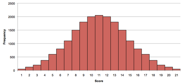
These data can be described according to a measure of central tendency, their spread and the shape of their distribution. The shape of the distribution is important in deciding upon the most appropriate method of description, and can be described according to skew (symmetry of the distribution) and kurtosis ('pointyness' of the distribution). A normal distribution (shown below) has a skew of zero and a kurtosis of zero, and is a very commonly used distribution in statistics. If data follow a normal distribution, then they can be completely described using only the mean and the standard deviation.
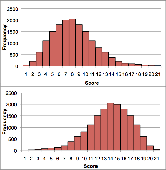
However, data may be skewed to the right (where there is a 'tail' on the right, also known as a positive skew) or to the left (where there is a 'tail' on the left, also known as a negative skew). In these cases, the observations in the tail can affect the estimate of the mean, and make it less useful as a measure of central tendency. This (and the lack of symmetry in the distribution) will also reduce the usefulness of the standard deviation as a measure of spread. In these cases, it is more appropriate to describe the data using the median and the interquartile range (as these measures are more robust against these extreme values).
In some cases (such as a bimodal distribution), the median may also not be an appropriate measure of central tendency, and the mode(s) may be more appropriate. This demonstrates that careful consideration of the usefulness of the available measures should be given whenever describing data, and 'common sense' should be used to select the most appropriate one. For example, although there is nothing statistically 'wrong' with using the mean to describe a highly skewed dataset, it does not offer the same amount of information as the median would do, and risks misrepresenting the data.

